Focus measurement on a microscope
Hullo, it’s been a while since the last post. I remember about the promise to finish the transponders writeup, bear with me for a bit longer.
Today is going to be something completely different: how to eastimate the best focus point on a motorized microscope. I won’t go into detail on what a motorized microscope is; suffice it to say it’s when you can just control all three axes programmatically.
So you want to image something with your ‘scope and probably you want the image to even be focused. Fair enough. It’s a challenge given that microscope objectives typically have a hilariously small depth of field, even the fine focusing knob requires minuscule motion on higher mag. Let me tell you how I went about it. Of course, that’s not the only or possibly not even the best solution, but it seems to work for me.
First of all, you want to have a general idea where your thing is, so we start with the target somewhat in focus. I am sure we all can get to that point somehow.
Then, I take a series of images while stepping the Z coordinate bit by bit, so the sample slowly goes into focus and then back – just like when you focus manually.
After that, the images can be processed to obtain a numerical measure of how badly things are out of focus. There are several approaches, it would appear, and some worked better than others for myself. Specifically, one fast and bad one is using the Canny algorithm to find “edges” in the images and then say just count them. It’s quick, easy to understand, and completely failing on 50x or better – at least on the ones I have: none of the images are sharp enough to trigger edge creation.
Failing that, I went for the slower candidate: the Laplacian. No idea what it actually does except it computes kinda the same thing, finding edges in the image. But here, we can get a continuous measure of sharpness as it is not like “edge or no edge” like Canny does but a nice and smooth function. With that, I can at least get a number for any of the images taken, no matter if it looks like you’re looking through frosted glass or if you have 20/20.
When plotted, things look like this:
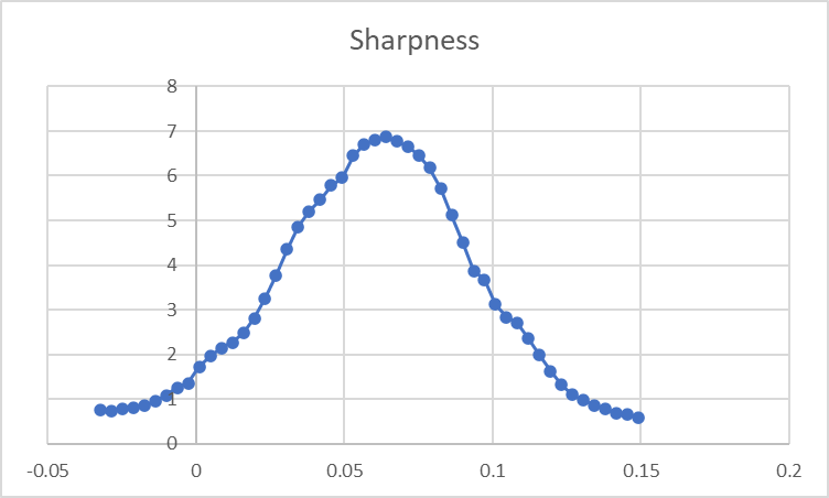
Now one could just say, ok, let’s just take the maximum and be happy with that. And that will work most of the time, indeed. But what we could do is take a proper approach and model this as a GAussian and try finding its parameters in the hope of being more precise; it could just happen that we don’t hit the maximum. Or, when the search range is large-ish, we could end up with only a few measurements standing out, leading to rather imprecise results. Oh, and we might want to do a round 2 in an attempt to further narrow things down – finding a good estimate for start and end Z values would help. I tried just dividing the coarse range by an integer and the results sucked.
After a ton of tries, I ended up with the following code piece:
import numpy as np
from scipy.optimize import curve_fit

def gauss(x, H, A, x0, sigma):
  return H + A * np.exp(-(x - x0) ** 2 / (2 * sigma ** 2))

def find_gaussian(points):
  # find a maximum to help with x0
  max_x = points[0][0]
  max_y = points[0][1]
  min_y = max_y
  for p in points:
    if max_y < p[1]:
      max_y = p[1]
      max_x = p[0]
    if min_y > p[1]:
      min_y = p[1]
  p0 = [min_y, max_y-min_y, 0, 1]
  # define parameter bounds to something sane
  bounds = (
    (0,       0,      points[ 0][0],  0),
    (np.inf,  np.inf, points[-1][0],  np.inf))
  # throw a fit
  x_data = [p[0] for p in points]
  y_data = [p[1] for p in points]
  parameters, covariance = curve_fit(gauss, x_data, y_data, p0=p0, bounds=bounds)
  return parameters # H, A, x0, sigma
First of all, we model our function. There is nothing surprising, just the good old bell-shaped thing.
Then, we try running the curve_fit function against our measurements. I found it is important to help it as much as possible to get good results (e.g. not ending with A negative, not ending with x0 outside the measured bounds, etc). With any luck, the returned x0 will be a more precise estimate for the Z than just the maximum. Then, we can use sigma to narrow the search range to e.g. x0 +- 2*sigma.
While there is no easy way to measure actual improvement, I am happy to have played with something new and getting results no worse than before.
XOXO, DJ